DOCSIS FBC (Full Band Capture) Impairment Algorithms - Wave

Feb 10

Written By Daniel Ratke | Software Engineer, Axiros GmbH

Wave Impairment

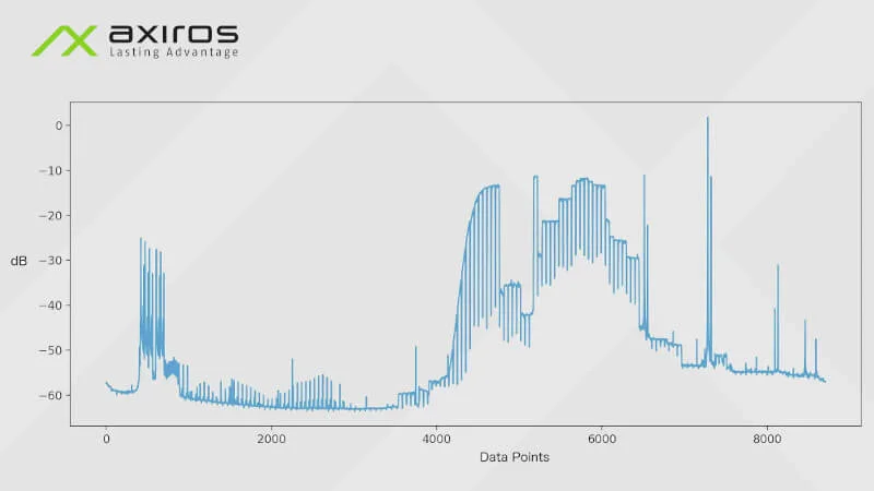
The wave impairment is one of many impairments that can be detected on a DOCSIS FBC (Full Band Capture) downstream spectrum. In the following, we take a cursory look at an implementation of the wave impairment detection algorithm. More theoretical information can be found in the official PNM guideline pdf by Cablelabs.

Before a potential wave impairment is fitted onto a spectrum, some data preparations are made. First and foremost, the data has to be stitched together. Only channels actually send data (these are the long, upside down U-shapes in the spectrum). Those channels are interpolated across the gaps with no data. The black line in the following picture shows how the algorithm stitches these channels together using linear regression.

DOCSIS FBC (Full Band Capture) Impairment Algorithms - Wave

A very simple and efficient linear regression implementation is given by scipy:

The above code is run for each gap that is found in the spectrum. The X and Y contain half of the channel before the gap and half of the channel after the gap. last_end and next_start denote the start and end of the gap.

Now, a wave impairment has some form of a sinusoidal curve. These curves can be analyzed using the FFT to get the composition of frequencies the given wave consists of. Thus, based on a smoothed version of the resulting data (using rolling averages) an inverse FFT (IFFT) is calculated. Below the result can be seen (this is also the main part of the algorithm).

Those huge impulses (denoted by a)) in the chart in 160 steps are the U-shapes (=channels). The algorithm guesses that harmonic based on the channel width and the spectrum width. They are supposed to decrease the higher the frequency. If they do not, if one of the impulses is bigger than the previous one, a wave impulse is detected. This is for waves that by coincidence fall exactly in the same frequency as the U shapes. If this was the case, the U shape would continue where there are no channels (just noise), even though with less power (height of the shape would be much smaller). These are called harmonic impulses.

Non-harmonic impulses, see b), are the ones that are on a different frequency than the guessed one. Most of the time, from what we have seen, they are less than 160 data points from the center. A significant impulse is one that has at least 45% the height of the last harmonic impulse. Now, all non-harmonic impulses that are higher than the last significant harmonic impulse are considered wave impulses.

In the previous section finding harmonics was not described in detail, but it is not as trivial as it may sound. What is a harmonic anyways? It is simply a local maximum of the data which repeats at the same distance. Thus, a harmonic search algorithm would have to get all local maxima (which require a hyperparameter, the 'locality' - how many data points to the left and right need to be less than a candidate point?) and find a period r that contains the most maxima. The harmonic with the most maxima is the harmonic of our channels. By the way, this harmonic could also be interpreted as a wave impairment, when it is obviously not - it is just our data channels. But this is dealt with at other places in the algorithm. For reference, the PNM guidelines pdf by Cablelabs mentions "[...] A DC term will be present. Comb teeth will be present every 166.67 ns due to the notch between 6 MHz channels". This describes exactly the harmonic of our channels.

Lastly, to deal with false-postives and false-negatives, a few additional constraints (mostly for edge cases) can be added. Note: The main harmonic is the first (and highest/most powerful) harmonic impulse. Now, the following three conditionals deal with wrong detections and thus increase the quality of predictions:

If more than 75% of all channels are flat, the candidate wave is ignored
Low frequency waves are ignored (below index 5, so a few hundred kHz)
Low power waves are ignored (if the amplitude is less than 70% of the main harmonic)

This wraps up the post. We have gotten a deeper look into the wave impairment detection algorithm used at Axiros. In summary, the algorithm has two major steps: Data preparation using linear regression and FBC spectrum analysis using FFT. Finally, we hope you could gain some insight into the wave impairment.

* The figures do not represent a product by Axiros, but merely show the algorithm.

From this blog series: